
Logistic Regression from Scratch on MNIST
Implementing binary logistic regression with gradient descent on 784-dimensional image data. Numerically stable gradients and learning rate tuning.
Abstract#
Binary logistic regression implemented from scratch with NumPy on an MNIST-like dataset (28x28 images, 784 features, ~6000 training samples). The gradient computation needed a numerical stability fix to avoid overflow. Tuned the learning rate over 10 values and picked the one with the lowest validation risk.
This was the first assignment where we had to implement an actual optimization loop instead of plugging into a closed-form solution. The dataset was a binary subset of MNIST — 28x28 pixel images flattened to 784-dimensional vectors, with labels and . About 6100 training samples, with separate validation and test splits provided.
The logistic loss#
The logistic regression risk function is:
This is the average log-loss. When is large and positive (correct prediction with high confidence), the loss for that sample is near zero. When it’s negative (wrong prediction), the loss grows linearly.
Gradient computation#
The gradient of the logistic loss with respect to is:
The problem is that can overflow when the product is a large negative number. With 784 features and float128 arithmetic, the dot products get big fast in early iterations when the weights are moving a lot.
The fix is to split the computation based on the sign of the product:
def calculate_gradient(w):
    gradient = np.zeros((1, 784), dtype=np.float128)
    for i in range(N):
        xi = trainingData[i]
        yi = trainingLabels[i]
        product = yi * np.dot(w, xi.T)

        if product >= 0:
            scalar = (-yi / N) * (np.exp(-product) / (1 + np.exp(-product)))
        else:
            scalar = (-yi / N) * (1.0 / (1 + np.exp(product)))

        gradient += scalar * xi
return gradientWhen product >= 0, is at most 1, so no overflow. When product < 0, we rewrite the fraction by multiplying numerator and denominator by , which gives . Now is also at most 1. Same value, no overflow either way.
Gradient descent#
Standard gradient descent. Initialize as zeros, iterate:
def gradient_descent(T, learning_rate):
    w = np.zeros((1, 784), dtype=np.float128)
    for t in range(T):
        grad = calculate_gradient(w)
        w = w - learning_rate * grad
return wNo momentum, no adaptive learning rate, no mini-batches. Full-batch gradient descent with a fixed step size. It’s slow (iterating over all 6107 samples per step, per sample), but the assignment wasn’t about speed.
Learning rate tuning#
I tested 10 learning rates with iterations each:
| Learning Rate | Training Risk | Validation Risk |
|---|---|---|
| 1e-6 | 0.1381 | 0.1454 |
| 5e-6 | 0.1125 | 0.1287 |
| 1e-5 | 0.1033 | 0.1260 |
| 2e-5 | 0.0946 | 0.1263 |
| 2.5e-5 | 0.0919 | 0.1270 |
| 3e-5 | 0.1207 | 0.1711 |
| 3.5e-5 | 0.0870 | 0.1328 |
| 5e-5 | 0.0866 | 0.1516 |
| 1e-4 | 0.1314 | 0.2754 |
| 1e-3 | 3.3060 | 5.2962 |
Learning rate 1e-5 had the lowest validation risk at 0.126. The training risk keeps going down with larger learning rates (down to 0.087 at 3.5e-5), but the validation risk starts climbing back up after 1e-5. That gap between training and validation risk is overfitting. The model fits the training data better but generalizes worse.
At 1e-3 everything blows up. The step size is too large and gradient descent overshoots, oscillating instead of converging. The risk of 5.3 on validation is worse than random guessing.
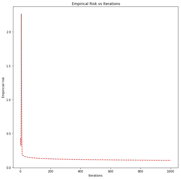
Empirical risk vs. iteration count for the best learning rate (1e-5). Monotonically decreasing, as expected for a convex loss with a small enough step size.
The risk curve is smooth and monotonically decreasing. Logistic loss is convex, so with a small enough learning rate you’re guaranteed to converge. No local minima to worry about.
Final model#
Using learning rate 1e-5 and :
- Validation risk: 0.126
- Test risk: 0.119
The test risk is slightly lower than the validation risk. Since I picked the learning rate based on validation performance, you’d expect validation to be slightly optimistic (we selected the model that happened to do best on validation), so the test risk being even lower is just noise from finite sample sizes. The two numbers are close enough that the model generalizes well.
For a linear model with no regularization on 784 features, this is a reasonable result. The logistic regression can only learn a linear decision boundary in the 784-dimensional pixel space, so there’s a ceiling on how well it can separate the two digit classes. The SVM models in the next assignment push that ceiling higher.