
Bayes vs LDA and VC Generalization Bounds
Comparing the Bayes-optimal quadratic boundary to Fisher LDA on 2D Gaussians, then testing VC dimension bounds on a rectangle concept learner.
Abstract#
Two problems. The first derives the Bayes decision boundary (quadratic, since the two classes have different covariances) and compares it to Fisher’s Linear Discriminant Analysis on the same test data. Both get 7% error, which was surprising. The second implements a rectangle concept learner and checks whether the empirical error stays below the VC generalization bound across many trials. It does.
Bayes boundary vs. Fisher’s LDA#
The setup is two 2D Gaussian classes:
- Class : mean , covariance
- Class : mean , covariance
The covariances are different, which means the Bayes-optimal boundary is quadratic, not linear. I generated 50 test points from each class.
Deriving the Bayes boundary#
When you set the log-posterior ratio to zero with unequal covariances, the quadratic terms from the Mahalanobis distances don’t cancel. The boundary I derived was:
np.random.seed(1)

mean_pos = [1, 0]
cov_pos = [[1, 0], [0, 1]]
p_x_y1 = np.random.multivariate_normal(mean_pos, cov_pos, 50)

mean_neg = [-1, 0]
cov_neg = [[1, -0.5], [-0.5, 1]]
p_x_y_minus1 = np.random.multivariate_normal(mean_neg, cov_neg, 50)

x1 = np.linspace(-4, 4, 100)
x2 = np.linspace(-4, 4, 100)
line = ((x1**2) / 3) + (14 * x1 / 3) + ((x2**2) / 3) + (4 * x2 / 3) + (4 * x1 * x2 / 3) + (1.0 / 3) - math.log(3)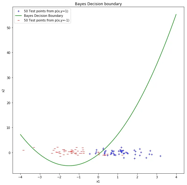
The Bayes decision boundary (green) separating the two classes. It’s a quadratic curve because the class covariances differ.
I classified each test point by evaluating the boundary expression and checking the sign. Test error: 7% (7 out of 100 points misclassified).
Fisher’s LDA#
LDA finds the projection direction that maximizes the ratio of between-class scatter to within-class scatter. The projection vector is:
where is the within-class covariance (the sum of the two class covariances estimated from training data).
np.random.seed(2)

# New training data for LDA (separate from test data)
train_pos = np.random.multivariate_normal(mean_pos, cov_pos, 50)
train_neg = np.random.multivariate_normal(mean_neg, cov_neg, 50)

mu_pos = np.mean(train_pos, axis=0)
mu_neg = np.mean(train_neg, axis=0)

cov_w_pos = np.cov(train_pos.T)
cov_w_neg = np.cov(train_neg.T)
c_w = cov_w_pos + cov_w_neg

w = np.linalg.inv(c_w).dot(mu_pos - mu_neg)The LDA boundary is linear: . I evaluated the same 100 test points against this boundary.
Test error for LDA: also 7%.
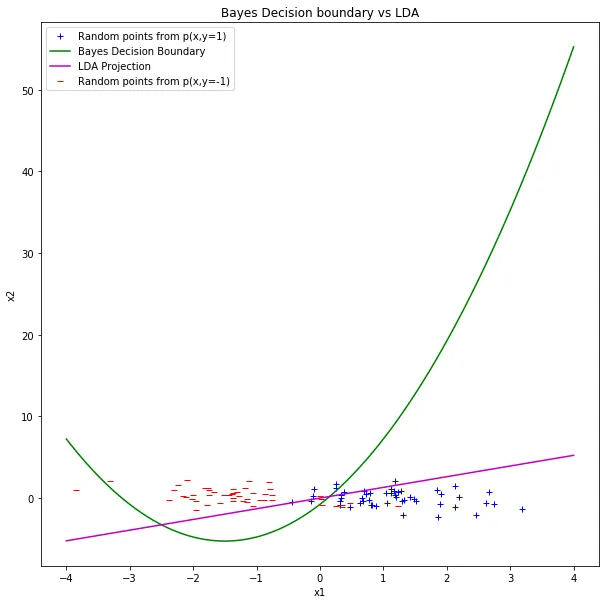
Bayes boundary (green) vs. LDA projection boundary (magenta). On this particular test set, they both achieve the same 7% error.
With only 50 test points per class, this could be coincidence. The Bayes boundary is the theoretical optimum, but the test set is small enough that LDA’s linear approximation doesn’t lose anything measurable. On a larger test set or with more separated covariances, you’d expect the quadratic boundary to pull ahead.
Rectangle concept learning and VC bounds#
The second problem was about generalization theory. The “true concept” is an axis-aligned rectangle inside the unit square . Points inside the rectangle are positive, points outside are negative.
The learner (Algorithm 1) sees labeled training points and outputs the largest rectangle that contains no negative points. Since it expands outward from the true rectangle until hitting the nearest negative sample on each side, it always produces a rectangle that’s at least as big as the true one. That means it can only make false positive errors on test data, never false negatives.
def find_largest_rectangle(x1_neg, x2_neg, l, r, b, t):
    # Expand each side to the nearest negative point
    l_largest = max([x for x, y in zip(x1_neg, x2_neg)
                     if x < l and b <= y <= t], default=0)
    r_largest = min([x for x, y in zip(x1_neg, x2_neg)
                     if x > r and b <= y <= t], default=1)
    b_largest = max([y for x, y in zip(x1_neg, x2_neg)
                     if y < b and l <= x <= r], default=0)
    t_largest = min([y for x, y in zip(x1_neg, x2_neg)
                     if y > t and l <= x <= r], default=1)
    return l_largest, r_largest, b_largest, t_largest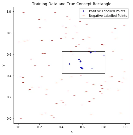
Training data in the unit square. Blue points are inside the true concept rectangle (black outline), red points are outside.
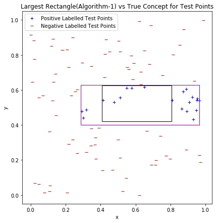
The learned rectangle (magenta) vs. the true concept rectangle (black) evaluated on test data. The learned rectangle is larger, so all errors are false positives.
The VC generalization bound#
Axis-aligned rectangles in 2D have VC dimension (four parameters: left, right, top, bottom). The generalization bound gives an upper limit on the true error:
where is the training error (0 in our case, since the learned rectangle never misclassifies training points), is the number of training samples, and (99% confidence).
I ran 100 trials for each of , , and , recording the test error each time.
| Theoretical bound | 99th percentile of test error | |
|---|---|---|
| 50 | 0.966 | 0.241 |
| 100 | 0.733 | 0.120 |
| 200 | 0.551 | 0.080 |
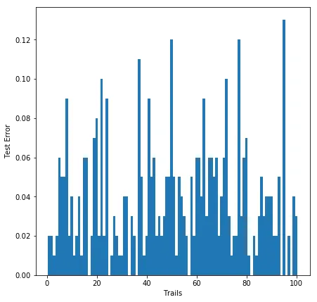
Distribution of test errors across 100 trials for . Most trials have low error, but there’s a long tail.
The 99th percentile of the empirical error is always well below the theoretical bound. The VC bound is famously loose. For the bound says error could be as high as 0.97 (almost useless), while the actual 99th percentile is 0.24. The bound gets tighter with more data, but it’s still conservative by a factor of 5-7x across all three sample sizes.
The point of the exercise wasn’t that the bound is tight. It’s that the bound holds. Across 100 random trials, the 99th percentile never exceeds the theoretical guarantee. That’s the whole promise of VC theory: a distribution-free upper bound that works regardless of what the true concept looks like.
The three things I took away:
- Test error decreases with larger , as you’d expect.
- The theoretical bound also decreases with , but much more slowly.
- The gap between theory and practice is large, but the bound never fails.