
Fractals for Image Classification Feature Extraction
Mapping images to a 1D signal with a Hilbert curve, compressing with wavelets, and classifying with SVMs on MNIST and Fashion-MNIST.
The idea#
CNNs dominate image classification, but the convolution operation is tightly coupled to a 2D pixel grid. I wanted to see what happens if you instead serialize the image into a 1D signal with a space-filling curve, compress it with a wavelet transform, and hand the result to an SVM. The hypothesis: a curve that preserves locality (the Hilbert curve) should retain enough spatial structure that a non-convolutional classifier can still do reasonably well.
This was a final-project writeup for an undergraduate ML course. The classifier is plain SVM, the dataset is MNIST and Fashion-MNIST, and the comparison is against the raw flattened image as a baseline.
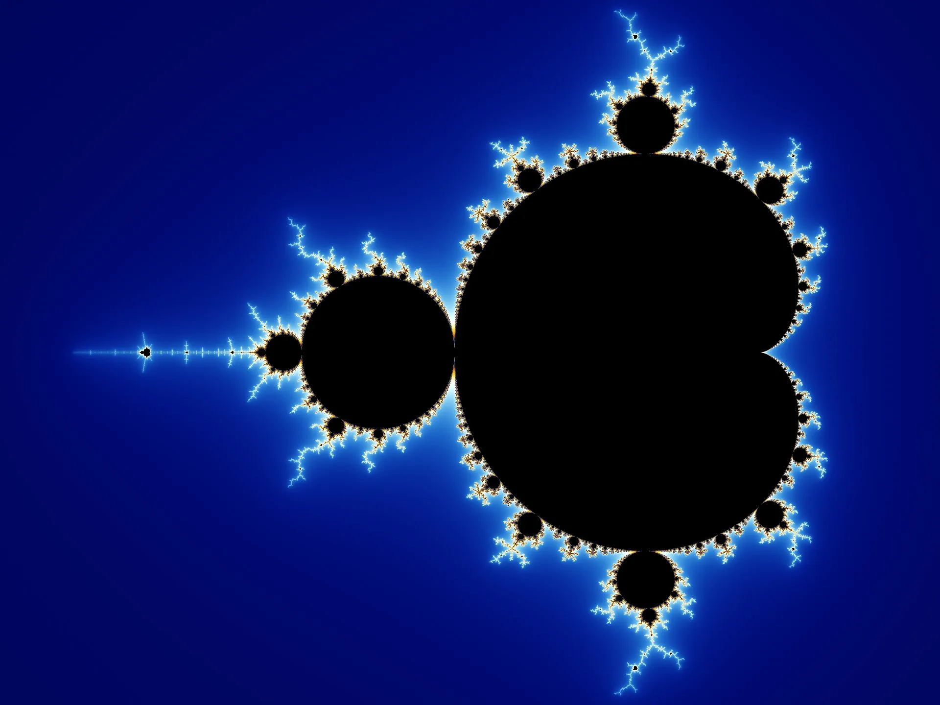
Fractals, briefly#
A fractal, in Mandelbrot’s definition, is a shape whose Hausdorff dimension is greater than its topological dimension. The Koch curve has topological dimension 1 and Hausdorff dimension 1.262. A rough surface might have topological dimension 2 and Hausdorff dimension 2.3.
For this project the relevant property is simpler: self-similar fractals can encode information from a higher dimension into a lower one. That property is what lossy image compression exploits, and it’s what I’m leaning on here.
Space-filling curves#
A space-filling curve traverses every point in a 2D (or higher-dimensional) region. The Hilbert curve is the standard example. Its finite approximations, called pseudo-Hilbert curves, are what get used in practice — for example, in devices that translate camera input into audio so that nearby pixels in the image map to nearby frequencies in the sound.
Comparing three curves#
Not all space-filling curves preserve locality equally well. I compared three: Z-curve (Morton order), Peano, and Hilbert. 1
Z-curve#
Easy to implement, but bad at locality. Adjacent points in the sequence often map to coordinates far apart in 2D. Average displacement for unit edges exceeds 1.6 in 2D and 1.35 in higher dimensions.Peano curve#
Better. Horizontal segments are exactly one unit, vertical segments can stretch to 2 or 5 units. Approaches the Hilbert curve's performance at higher ranks.Hilbert curve#
The best of the three. Adjacent points in the 1D sequence are also adjacent in 2D, and the property holds across resolutions and dimensions. This is what I used.Hilbertification#
I’ll call the mapping process “Hilbertification”: take an image, traverse it along a Hilbert curve, and emit the pixel intensities in traversal order. The result is a 1D sequence where neighboring values correspond to neighboring pixels in the original image.
The construction is recursive:
- Divide the image into quadrants and define a traversal order.
- Subdivide each quadrant and apply the same pattern, oriented appropriately.
- Continue until every pixel has been visited.
The output is a 1D vector of length width × height whose ordering reflects the curve’s path.
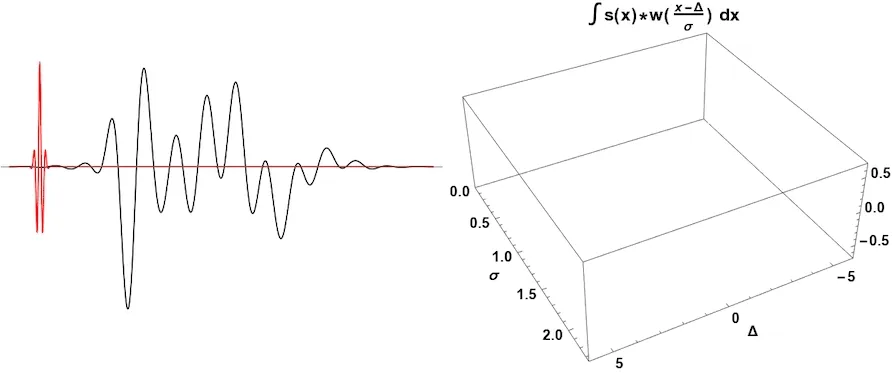
Wavelet transform for compression#
After Hilbertification I apply a wavelet transform. Wavelets give both frequency and spatial localization, unlike a plain Fourier transform which only gives frequency. For a 1D signal this is just a standard discrete wavelet decomposition; I kept the approximation coefficients and dropped the detail coefficients at one level, which cuts the feature dimension to roughly one-quarter of the original image.
Classifier#
The classifier is an SVM. SVMs are a reasonable choice here because they handle high-dimensional input well and the kernel trick lets me try a few decision-boundary geometries (linear, RBF, polynomial) on the same features. 2
The pipeline:
- Flatten the image (or Hilbertify and wavelet-compress it).
- Train one SVM per kernel choice.
- Evaluate on the test set.

Results#
Baseline is the raw flattened image. Hilbertified is after the curve traversal and wavelet step, which is about one-quarter the feature dimension.
| Dataset | Method | Linear SVM | RBF Kernel | Polynomial Kernel |
|---|---|---|---|---|
| Fashion MNIST | Hilbertified | 87.27 | 88.28 | 87.99 |
| Baseline | 91.49 | 89.92 | 91.58 | |
| MNIST | Hilbertified | 96.03 | 96.54 | 97.13 |
| Baseline | 98.32 | 98.66 | 99.29 |
A few notes on what didn’t work and what I didn’t get to:
- I also tried feeding the SVM cosine-transformed features as another baseline. Accuracy was abnormally low, almost certainly a bug in my transform code. I didn’t include those numbers in the table.
- I wanted to extend the method to CIFAR-10, but that’s a color dataset and I ran out of time to adapt the pipeline for three channels.
What I take away#
The Hilbertified features hold up. Accuracy drops a few percentage points on Fashion-MNIST (4 points worst case) and about 2 points on MNIST, in exchange for a 4× reduction in feature dimensionality. That’s a useful trade if your downstream constraint is memory or training time rather than peak accuracy.
The more interesting result is that the locality-preserving curve carries enough spatial structure for a non-convolutional classifier to land within a few points of the raw-pixel baseline. The wavelet step is doing some of the work, but the locality property of the Hilbert curve is what makes the wavelet meaningful — without it you’d be wavelet-transforming an arbitrary pixel ordering.
The natural extension is higher-dimensional inputs: video, volumetric medical scans, anything where the data has more than two spatial axes. The Hilbert construction generalizes to any number of dimensions and the locality property holds, so the same pipeline should drop in.
Footnotes#
-
Jaffer, Aubrey. “Color-Space Dimension Reduction.” Accessed November 19, 2018. https://people.csail.mit.edu/jaffer/CNS/PSFCDR ↗. ↩
-
Alex J. Smola, Bernhard Scholkopf. “A Tutorial on Support Vector Regression.” Statistics and Computing archive Volume 14 Issue 3, August 2004, p. 199-222. ↩