
NCC Template Matching, Stereo Depth, and KNN
NCC template matching on a Simpsons scene, brute-force stereo depth from two views, and k-nearest neighbors classification.
Abstract#
Three problems. The first implements normalized cross-correlation template matching to find Stampy the elephant in a crowded Simpsons scene, using FFT convolution and integral images for speed. The second computes a stereo depth map from a pair of images by brute-force NCC at every pixel (four nested Python for-loops; it was slow). The third is k-nearest neighbors classification on a 2D dataset using sklearn.
Part 1: Template matching (NCC)#
The search image is a crowded scene from The Simpsons, and the template is a crop of “Stampy” the elephant. NCC works by sliding the template across the image and computing normalized cross-correlation at each position. High NCC = good match.
Load both and convert the search image to float64:
search = imread('./data/search.png')
template = imread('./data/template.png')
image = np.array(search, dtype=np.float64, copy=False)Pad the image with zeros by the template shape on all sides so we can slide the template without going out of bounds.
pad_width = tuple((width, width) for width in template.shape)
image = np.pad(image, pad_width=pad_width, mode='constant', constant_values=0)Efficient window sums#
Computing NCC at every position requires the sum and sum-of-squares of pixels in each template-sized window. I used cumulative sums along each axis (the integral image idea, extended to 3D since the image has color channels).
def calc_window_sum(image, window_shape):
    window_sum = np.cumsum(image, axis=0)
    window_sum = (window_sum[window_shape[0]:-1]
                  - window_sum[:-window_shape[0] - 1])
    window_sum = np.cumsum(window_sum, axis=1)
    window_sum = (window_sum[:, window_shape[1]:-1]
                  - window_sum[:, :-window_shape[1] - 1])
    window_sum = np.cumsum(window_sum, axis=2)
    window_sum = (window_sum[:, :, window_shape[2]:-1]
                  - window_sum[:, :, :-window_shape[2] - 1])
return window_sumThree passes of cumsum-and-subtract, one per axis.
image_window_sum = calc_window_sum(image, template.shape)
image_window_sum2 = calc_window_sum(image ** 2, template.shape)Cross-correlation via FFT#
Cross-correlation in spatial domain is convolution with a flipped kernel. fftconvolve does it in the frequency domain, faster for large templates.
template_mean = template.mean()
template_volume = np.prod(template.shape)
template_ssd = np.sum((template - template_mean) ** 2)

xcorr = fftconvolve(image, template[::-1, ::-1, ::-1],
mode="valid")[1:-1, 1:-1, 1:-1][::-1, ::-1, ::-1] flips the template along all three axes, and the [1:-1, ...] trims an extra border pixel from the valid output.
NCC formula#
The numerator and denominator are computed over the whole image at once:
numerator = xcorr - image_window_sum * template_mean

denominator = image_window_sum2
image_window_sum = np.multiply(image_window_sum, image_window_sum)
image_window_sum = np.divide(image_window_sum, template_volume)
denominator -= image_window_sum
denominator *= template_ssd
denominator = np.maximum(denominator, 0)  # clamp before sqrt
denominator = np.sqrt(denominator)Division only happens where the denominator is above machine epsilon. Everything else stays zero.
response = np.zeros_like(xcorr, dtype=np.float64)
mask = denominator > np.finfo(np.float64).eps
response[mask] = numerator[mask] / denominator[mask]Then crop the response back to the original image dimensions:
slices = []
for i in range(template.ndim):
    d0 = template.shape[i] - 1
    d1 = d0 + image_shape[i] - template.shape[i] + 1
    slices.append(slice(d0, d1))
result = response[tuple(slices)]Finding the top matches#
np.argpartition is faster than a full sort when you only need the top N:
def largest_indices(ary, n):
    """Returns the n largest indices from a numpy array."""
    flat = ary.flatten()
    indices = np.argpartition(flat, -n)[-n:]
    indices = indices[np.argsort(-flat[indices])]
return np.unravel_index(indices, ary.shape)I tested the 1st, 2nd, 5th, 10th, 100th, and 500th best matches. One thing that bit me here:
ij = np.unravel_index(np.argmax(result), result.shape)
_, x, y = ij[::-1]
# IMPORTANT TO SWITCH ROWS AND COLUMNS
# I've LOST 5 points this semester because of thisNumPy’s unravel_index returns (row, col) order but matplotlib’s Rectangle and image indexing expect (x, y). I kept forgetting to swap them and losing points on earlier assignments. By HW9 I’d finally burned this into my brain enough to leave myself an all-caps comment.
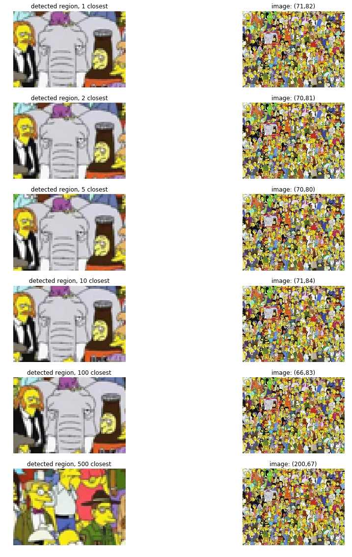
The top 1 through 10 matches all land on Stampy almost pixel-for-pixel. The 2nd and 5th closest are only off by 1-2 pixels, basically indistinguishable. By the 100th match, it drifts too far left: you can see more of John Swartzwelder (the guy in the suit) and Brandine (the lady on the right) has disappeared from the crop. By the 500th match, we’re closer to Homer than to Stampy. Way off.
Part 2: Stereo depth via template matching#
Given a left and right image of the same scene (grayscale stereo pair), compute a depth map. Closer objects have larger horizontal disparity between the two views, so if you can measure that disparity per-pixel, you get depth.
left = imread('./data/left.png')
right = imread('./data/right.png')Brute force: for every pixel in the left image, extract a window around it, slide that window horizontally across the right image (up to max_offset pixels), and compute NCC at each offset. Whichever offset gives the highest NCC is the estimated disparity.
def stereo_match(left_img, right_img, kernel=11, max_offset=50):
    w, h = left_img.shape
    depth = np.zeros((w, h), np.uint8)
    depth.shape = h, w
    kernel_half = kernel // 2
    offset_adjust = 255 / max_offset

    for y in range(kernel_half, h - kernel_half):
        for x in range(kernel_half, w - kernel_half):
            best_offset = 0
            prev_ncc = float("-inf")

            for offset in range(max_offset):
                ncc = 0
                lwindow = left[y-kernel_half:y+kernel_half,
                               x-kernel_half:x+kernel_half]
                rwindow = right[y-kernel_half:y+kernel_half,
                                x-kernel_half:x+kernel_half]
                lwindow_mean = lwindow.mean()
                lwindow_std = np.std(lwindow)
                rwindow_mean = rwindow.mean()
                rwindow_std = np.std(rwindow)

                for v in range(-kernel_half, kernel_half):
                    for u in range(-kernel_half, kernel_half):
                        ncc_temp = ((int(left[y+v, x+u]) - lwindow_mean)
                                    * (int(right[y+v, (x+u) - offset])
                                       - rwindow_mean))
                        if lwindow_std == 0 or rwindow_std == 0:
                            ncc_temp = 0
                        else:
                            ncc_temp /= lwindow_std * rwindow_std
                        ncc += ncc_temp

                if ncc > prev_ncc:
                    prev_ncc = ncc
                    best_offset = offset

            depth[y, x] = best_offset * offset_adjust

return depthFour nested Python for-loops. It ran, but it was slow. I probably should have vectorized the inner loops with NumPy, or at least the kernel summation. But it did produce a depth map.
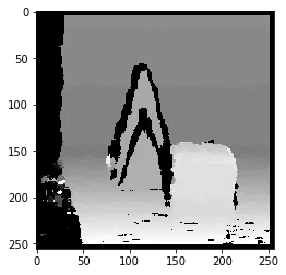
You can make out the shape of a person. Background is darker (smaller disparity, farther away), the figure is brighter.
Part 3: k-Nearest Neighbors#
2D points with class labels, two classes. Train on one set, predict on another.
train = np.loadtxt('./data/train.txt')
test = np.loadtxt('./data/test.txt')
X_train, y_train = train[:, 0:2], train[:, 2]
X_test, y_test = test[:, 0:2], test[:, 2]I used sklearn.neighbors.KNeighborsClassifier and tested :
neighbours = [1, 5, 11, 15]

f, axarr = plt.subplots(2, 2, sharex='col', sharey='row', dpi=150)
for n in neighbours:
    idx = neighbours.index(n)
    model = KNeighborsClassifier(n_neighbors=n)
    model.fit(X_train, y_train)
    y_pred = model.predict(X_test)
    cmap_bold = ListedColormap(['#FF0000', '#00FF00', '#0000FF'])

    axarr[idx//2, idx%2].scatter(X_test[:, 0], X_test[:, 1],
                                  c=y_pred, cmap=cmap_bold, s=1)
    axarr[idx//2, idx%2].scatter(
        X_test[y_pred != y_test, 0],
        X_test[y_pred != y_test, 1],
        c='#00FF00', edgecolor='k', cmap=cmap_bold, s=10)
    axarr[idx//2, idx%2].set_title(
        f"$k$={n}, Acc={round(model.score(X_test, y_test)*100, 2)}%")
plt.show()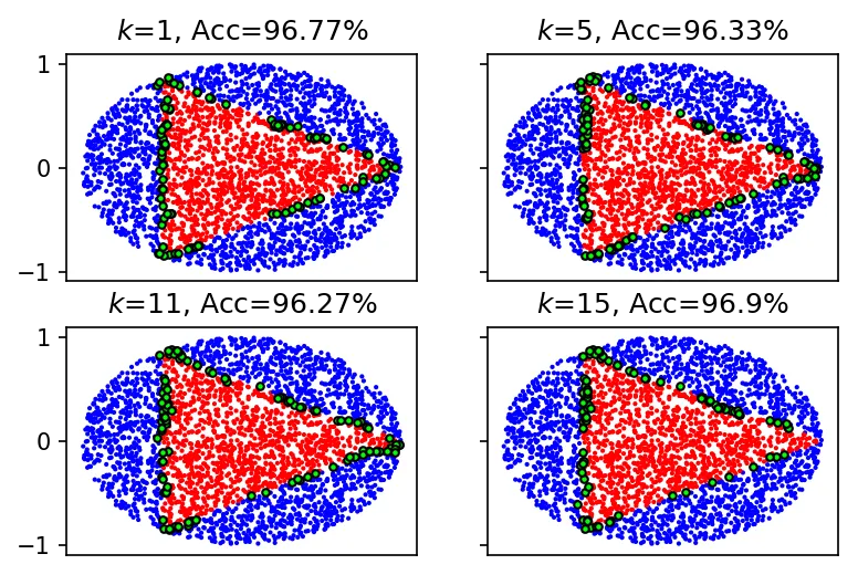
Accuracies: is 96.77%, is 96.33%, is 96.27%, is 96.9%.
The errors are all at the boundary between the two classes, where the nearest neighbors are a mix of both. Accuracy dips going from to , then jumps back up at . I think at small values, adding neighbors pulls in wrong-class points right at the boundary. At you’re sampling enough of the local area that the majority vote is more representative.
Not much code to write for this part since sklearn does all the work.