Camera Calibration and Homography

Abstract#

Two applications of the Direct Linear Transform. The first recovers a 3x4 camera projection matrix from 100 known 2D-3D point correspondences. The second estimates a 3x3 homography from 15 point pairs using the normalized DLT, which conditions the data before solving to reduce numerical error. Both are solved via eigendecomposition of $A^T A$.

Camera calibration (DLT)#

We have 100 3D world points and their corresponding 2D image coordinates. We want the 3x4 projection matrix $P$ such that

$x = PX$

where $X$ is a homogeneous 3D point $[X, Y, Z, 1]^T$ and $x$ is the projected 2D point $[u, v, 1]^T$ (in homogeneous coordinates, so we divide by the third component after projecting).

Load the data:

x = np.loadtxt('./data/2Dpoints.txt')  # 100x2
X = np.loadtxt('./data/3Dpoints.txt')  # 100x3

Building the system#

Each point correspondence gives us two equations (one for $u$, one for $v$). With 100 points that’s 200 equations for 12 unknowns (the entries of the 3x4 matrix $P$). I built the system by constructing three blocks t1, t2, b, each of size $(200 \times 4)$:

t1 = np.zeros((2*len(X), 4))
t2 = np.zeros((2*len(X), 4))
b = np.zeros((2*len(X), 4))
for i in range(len(X)):
    xi, yi = x[i]
    t1[i*2] = np.hstack((X[i], [1]))
    t2[i*2+1] = np.hstack((X[i], [1]))
    b[i*2] = np.hstack((-xi*X[i], [-xi]))
    b[i*2+1] = np.hstack((-yi*X[i], [-yi]))

Even rows put the homogeneous 3D point in t1 with zeros in t2. Odd rows do the reverse. The b block has $-u_i [X_i, Y_i, Z_i, 1]$ in even rows and $-v_i [X_i, Y_i, Z_i, 1]$ in odd rows. Stack them horizontally:

A = np.hstack((t1, t2, b))  # 200x12

This gives us $A\mathbf{p} = 0$ where $\mathbf{p}$ is the 12-element vector we want to recover.

Solving#

Eigendecompose $A^T A$, take the eigenvector with the smallest eigenvalue, normalize it to unit norm, reshape to 3x4.

ew, ev = np.linalg.eig(A.T @ A)
p = ev[:, np.argmin(ew)]
p /= np.linalg.norm(p)
p = p.reshape((3, 4))

Projecting back#

To check, project the 3D points through our recovered $P$ and divide by the third coordinate to get back to 2D:

out_proj = (p @ np.hstack((X, np.ones((len(X), 1)))).T).T
out_proj[:, 0] = out_proj[:, 0] / out_proj[:, 2]
out_proj[:, 1] = out_proj[:, 1] / out_proj[:, 2]

The projected points were slightly off from the originals. Some were way off, outside the input domain entirely. I thought clamping the output to the input domain might help the error, but it’s unclear how much that would mess with the semantics of the projection.

Sum of squared error: 18.75.

Homography (normalized DLT)#

This part maps between two sets of 2D points instead. 15 point correspondences from a file, and we want the 3x3 homography $H$ mapping points from image 1 to image 2.

The data file was comma-separated with four values per line (x1, y1, x2, y2). np.loadtxt() didn’t like the format, so I wrote a small parser:

def fileprocess(s):
    im1, im2 = [], []
    with open(s) as file:
        for line in file:
            a, b, c, d = line.split(',')
            im1.append([float(a), float(b)])
            im2.append([float(c), float(d)])
    return im1, im2

img1, img2 = fileprocess('./data/homography.txt')
img1, img2 = np.array(img1), np.array(img2)

Normalization#

The “normalized” in normalized DLT is about conditioning the data before solving. Translate each point set so its centroid is at the origin, then scale so the average distance from the origin is $\sqrt{2}$.

The normalization matrix $T$ for a point set is:

$T = \begin{bmatrix} s & 0 & -s\bar{x} \\ 0 & s & -s\bar{y} \\ 0 & 0 & 1 \end{bmatrix}$

where the scale factor is:

$s = \frac{\sqrt{2}}{\text{mean}\left(\sqrt{(x - \bar{x})^2 + (y - \bar{y})^2}\right)}$

def computeTransform(img):
    x = img[:, 0]
    y = img[:, 1]
    T = np.zeros((3, 3))

    s = np.sqrt(2) / np.mean(np.sqrt((x - x.mean())**2 + (y - y.mean())**2))

    T[0] = np.array([s, 0, -s*x.mean()])
    T[1] = np.array([0, s, -s*y.mean()])
    T[2] = np.array([0, 0, 1])

    return T, s

Ta, s1 = computeTransform(img1)
Tb, s2 = computeTransform(img2)

The normalize function subtracts the mean and multiplies by the scale:

def normalize(img, s):
    img2 = np.zeros(img.shape)
    x = img[:, 0] - img[:, 0].mean()
    y = img[:, 1] - img[:, 1].mean()
    img2[:, 0] = s * x
    img2[:, 1] = s * y
    return img2

img1_n = normalize(img1, s1)
img2_n = normalize(img2, s2)

Computing $\tilde{H}$#

Same DLT idea as before, just 3x3 instead of 3x4. Build three blocks ht1, ht2, ht3, each $(30 \times 3)$, using the normalized coordinates:

ht1 = np.zeros((2*len(x1), 3))
ht2 = np.zeros((2*len(x1), 3))
ht3 = np.zeros((2*len(x1), 3))
for i in range(len(x1)):
    ht1[i*2] = np.hstack((x1[i], y1[i], 1))
    ht2[i*2+1] = np.hstack((x1[i], y1[i], 1))
    ht3[i*2] = np.hstack((-x2[i]*x1[i], -y1[i]*x2[i], -x2[i]))
    ht3[i*2+1] = np.hstack((-y2[i]*x1[i], -y1[i]*y2[i], -y2[i]))

AH_bar = np.hstack((ht1, ht2, ht3))  # 30x9

Solve the same way. Eigendecompose $\bar{A}_H^T \bar{A}_H$, smallest eigenvector, normalize, reshape to 3x3:

ew2, ev2 = np.linalg.eig(AH_bar.T @ AH_bar)
H_bar = ev2[:, np.argmin(ew2)]
H_bar /= np.linalg.norm(H_bar)
H_bar = H_bar.reshape((3, 3))

Denormalization#

$\tilde{H}$ maps between normalized coordinates. To get the homography in original coordinates, undo the normalization:

$H = T_b^{-1} \tilde{H} T_a$

H = np.linalg.inv(Tb).dot(H_bar).dot(Ta)

Projection and comparison#

Run the image 1 points through $H$, divide by the third coordinate:

img2_proj = (H.dot(np.hstack((img1, np.ones((len(img1), 1)))).T)).T
img2_proj[:, 0] = img2_proj[:, 0] / img2_proj[:, 2]
img2_proj[:, 1] = img2_proj[:, 1] / img2_proj[:, 2]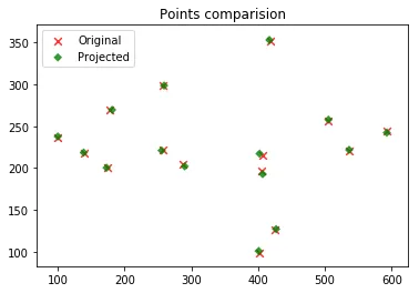

The projected points follow the same trend as the originals but are off by a bit. I figured a least squares fit instead of DLT might do better. Could also try different numerical methods for solving the system and compare.

Sum of squared error: 105.97.

Compared to the camera calibration error of 18.75, this is a lot worse, but we also only had 15 correspondences instead of 100.