Finding Edges with Gaussians, Sobel, and Canny
Gaussian smoothing, implementing derivative filters from scratch, Sobel vs Canny, and making Keanu Reeves look like A Scanner Darkly.
Abstract#
This assignment covered the basics of image filtering and edge detection. I implemented a Gaussian derivative filter from scratch (the 2D version first, then a separable 1D version when the 2D one wouldn’t cooperate with skimage), applied Sobel and Canny edge detectors to a grayscale photo of Keanu Reeves, and compared the results. The bonus at the end uses segmentation to approximate the cel-shading look from A Scanner Darkly.
Gaussian smoothing#
First part: blur Keanu at different sigma values and figure out when he stops being recognizable. I picked the sigmas by trial and error with some friends. We’d look at each blurred version and say whether we could tell who it was.
sigmas = [20, 15, 12, 10, 1, 0.5]

f, axarr = plt.subplots(2, 3, sharex='col', sharey='row', dpi=200)
for sigma in sigmas:
    filteredIm = gaussian(keanu, sigma)
    idx = sigmas.index(sigma)
    axarr[int(idx/3), idx%3].axis('off')
    axarr[int(idx/3), idx%3].set_title(f'$\\sigma$ = {sigma}')
    axarr[int(idx/3), idx%3].imshow(filteredIm, cmap='gray', aspect='auto')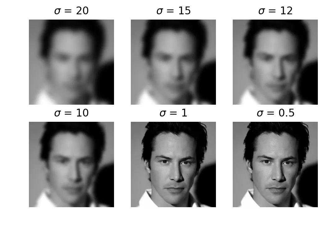
Keanu at sigma = 20, 15, 12, 10, 1, 0.5
The sigmas don’t follow any kind of scale. was where people disagreed. Some friends could still tell it was Keanu, others had no idea. Below nobody noticed any difference from the original.
One MATLAB thing worth noting: the homework document referenced fspecial() for building Gaussian kernels, which takes the kernel size as an argument. That function is deprecated now in favor of imgaussfilt(). On the Python side, skimage.filters.gaussian() wraps scipy.ndi.gaussian() and handles the kernel size automatically. I just passed sigma and let it figure out the rest.
Gaussian derivative filter#
The assignment wanted us to compute 2D Gaussian derivative masks. From the class notes:
I wrote the naive 2D kernel first:
def gaussX(sigma):
    l = 2 * sigma + 1
    ax = np.arange(-l, l)
    xx, yy = np.meshgrid(ax, ax)
    kernel = -(xx * np.exp(-(xx**2 + yy**2) / (2. * sigma**2))) / (2*math.pi * (sigma**4))
    kernel = kernel / np.sum(kernel)
return kernelWriting the filter itself was easy enough. Applying it was the problem. The way skimage processes things, wiring this kernel into sklearn.ndi.generic_filter was a pain. I spent a while on it and gave up.
In class we’d talked about how you can split a 2D Gaussian into two 1D passes. I went with that instead. You build a 1D Gaussian kernel, multiply by to get the derivative, and apply it along each axis with scipy.ndimage.filters.correlate1d. Applying along one axis and transposing gives you .
from scipy.ndimage.filters import correlate1d

def gaussian_derivative_filter1d(input, sigma, axis=-1, output=None,
                                  mode="reflect", cval=0.0, truncate=4.0):
    sd = float(sigma)
    lw = int(truncate * sd + 0.5)
    weights = [0.0] * (2 * lw + 1)
    weights[lw] = 1.0
    sum = 1.0
    sd = sd * sd

    # build gaussian kernel
    for ii in range(1, lw + 1):
        tmp = math.exp(-0.5 * float(ii * ii) / sd)
        weights[lw + ii] = tmp
        weights[lw - ii] = tmp
        sum += 2.0 * tmp
    for ii in range(2 * lw + 1):
        weights[ii] /= sum

    # first order derivative
    weights[lw] = 0.0
    for ii in range(1, lw + 1):
        x = float(ii)
        tmp = -x / sd * weights[lw + ii]
        weights[lw + ii] = -tmp
        weights[lw - ii] = tmp

return correlate1d(input, weights, axis, output, mode, cval, 0)More code than the naive version, but it actually works with the library and runs faster.
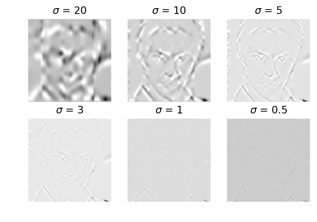
Gaussian derivative magnitude at sigma = 20, 10, 5, 3, 1, 0.5
The cmap='gray' display is a little wonky here because of float-to-int conversion, but you can see the edges. Lower sigma = more detail and more noise. Higher sigma = broad strokes only.
Thresholding#
Take the derivative output at , normalize to [0, 255], and threshold at different levels.
from sklearn.preprocessing import normalize

magIm = gaussDeriveApplyFilter(keanu, sigma=3)
magIm = normalize(magIm, axis=0, norm='max') * 255.0

threshLevels = [25, 50, 75, 125, 175, 225]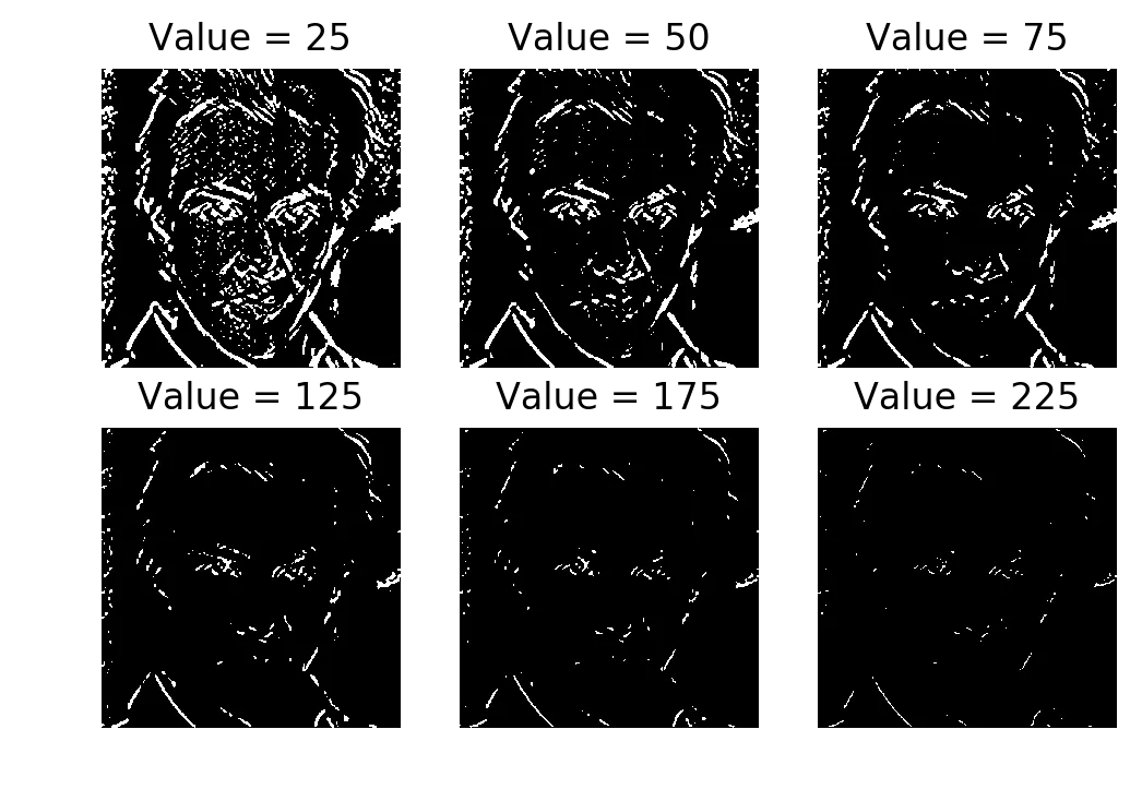
Thresholded at 25, 50, 75, 125, 175, 225
Threshold = 50 gives you a semi-decent edge image, but it’s grainy. There are specks of activation on the forehead, for example. I think that’s precision round-off from computing the Gaussian manually. The Sobel operator (next section) doesn’t have this problem, probably because its kernel uses integer values.
Sobel comparison#
from skimage.filters import sobel

edges1 = sobel(keanu)
edges2 = sobel(gaussian(keanu, sigma=3))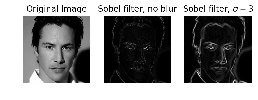
Original, Sobel without blur, Sobel with blur (sigma=3)
Sobel gives finer, smoother edge lines than my Gaussian derivative filter. I tried blurring the image first (sigma=3) before applying Sobel, expecting the edges to become more continuous. They didn’t. The blur just made the existing edges thicker.
Canny edge detector#
from skimage import feature

edges1 = feature.canny(keanu)
edges2 = feature.canny(keanu, sigma=3)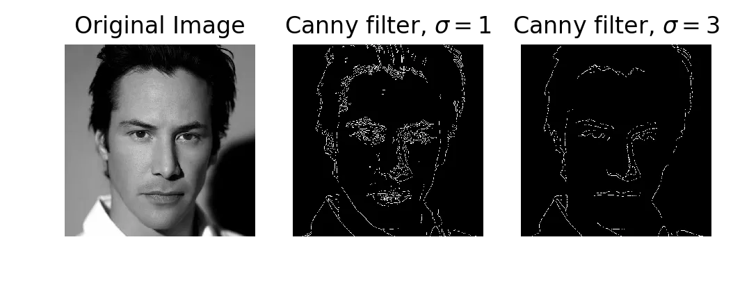
Original, Canny at sigma=1, Canny at sigma=3
Canny is the one that gives you continuous contour lines. With Sobel and with my Gaussian derivative filter, edges are broken up. Canny connects them. Increasing sigma to 3 drops the smaller features (eyebrow hairs, tufts of hairline) but the contours stay connected.
The reason is that Canny does non-maximum suppression and hysteresis thresholding after computing the gradient. Sobel and raw Gaussian derivatives just give you gradient magnitudes. You’re on your own for thresholding those.
Bonus: etch-a-sketch#
The homework was done at this point. I wanted to try some things with what we’d covered.
Sobel + Otsu threshold + invert on a color image. The blur beforehand makes the edges thicker, which controls the “pencil width.”
from skimage.color import rgb2gray
from skimage.util import invert
from skimage.filters import sobel, threshold_otsu

keanu_colour = imread('keanu_colour.jpg')
blur_keanu = gaussian(keanu_colour)
clean_keanu = rgb2gray(blur_keanu)
edge_keanu = sobel(clean_keanu)
thresh_mesh = threshold_otsu(edge_keanu)
binary_keanu = edge_keanu > thresh_mesh

plt.imshow(invert(binary_keanu), cmap='gray')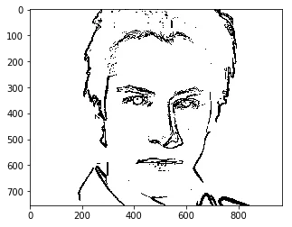
Sobel + Otsu + invert = pencil sketch
Bonus: A Scanner Darkly#
The movie A Scanner Darkly uses cel-shading, which needs 3D surface normals to compute. We don’t have 3D data here, but you can get something in the same neighborhood with image segmentation.
Quickshift segmentation breaks the image into superpixels. Build a region adjacency graph (RAG) based on mean color, merge regions with similar colors using cut_threshold, and draw the segment boundaries in black on top of the averaged colors.
from skimage import segmentation, color
from skimage.future import graph

keanu_colour = imread('keanu_colour.jpg')

labels1 = segmentation.quickshift(keanu_colour, kernel_size=7,
                                   max_dist=6, ratio=0.5)
out1 = color.label2rgb(labels1, keanu_colour, kind='avg')

g = graph.rag_mean_color(keanu_colour, labels1)
labels2 = graph.cut_threshold(labels1, g, 20)
out2 = color.label2rgb(labels2, keanu_colour, kind='avg')
out2 = segmentation.mark_boundaries(out2, labels2, (0, 0, 0))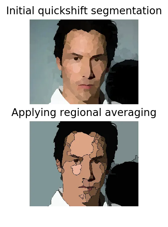
Quickshift segmentation (top), then RAG merging with boundaries drawn (bottom)
More simplistic than the actual cel-shading from the movie. The cut_threshold parameter (20 here) controls how aggressively regions get merged. Lower values = more segments. Higher values = big flat color blobs.
What I got out of this#
The Gaussian derivative implementation was most of the work. The naive 2D kernel is easy to write but I couldn’t get it to play nice with skimage’s API. The separable 1D version is more code but it actually fits into the library.
For the edge detector comparison: my Gaussian derivative filter gives rough edges with noise. Sobel cleans that up. Canny gives connected contours. They all start with the same idea (convolve with a derivative kernel) but Canny does extra work on top of the gradient computation to link edges together.