Ensembles, PCA, and K-Means on MNIST
Gradient descent for kernel learning, decision tree ensembles with bagging and boosting, PCA eigendigits, and k-means clustering on handwritten digits.
Abstract#
Gradient descent for kernel learning, decision trees with bagging and AdaBoost, PCA with eigendigit visualization, and k-means clustering with varying cluster counts, all applied to MNIST 7 vs 9 digit classification.
This was the third and final homework for statistical machine learning. Same MNIST 7-vs-9 dataset as the previous two assignments (2000 training images, 2000 test images, 784 pixels each). The problems here are less about theory and more about throwing different methods at the same data and seeing what sticks. We go from iterative kernel solvers to ensemble methods to unsupervised learning, and the results tell a nice story about what each approach can and can’t do.
Gradient descent for kernel learning#
In the previous homework we solved the kernel least squares problem by directly inverting the regularized kernel matrix: . That works, but matrix inversion is . An alternative is gradient descent (specifically, Richardson iteration), which avoids the inversion entirely.
The idea is simple. We want to minimize:
The gradient is , but for Richardson iteration we just use the simpler update:
where is the learning rate. This converges to the same solution as the direct method, just iteratively.
Using the Gaussian kernel from HW2 with and a learning rate of :
def iterative(n):
    K1 = np.zeros([2000, 2000], dtype=float)
    for i in range(2000):
        for j in range(2000):
            K1[i,j] = GaussianKernel(
                data_scaled_shuffle[i,:],
                data_scaled_shuffle[j,:],
                final_sigma2
            )

    learning_rate = 1e-3
    alphas = np.zeros(2000)

    for i in range(n):
        alphas = alphas - learning_rate * (
            np.matmul(K1, alphas) - output_shuffle
        )

    # Evaluate on test set
    cnt = 0
    for i in range(2000):
        pred = sum(
            alphas[j] * GaussianKernel(
                data_scaled_shuffle[j,:],
                data_test_scaled[i,:],
                final_sigma2
            )
            for j in range(2000)
        )
        if (pred >= 0) == (y[i] == 1):
            cnt += 1
return cnt / 2000| Iterations | Test accuracy |
|---|---|
| 2 | 91.25% |
| 5 | 92.65% |
| 10 | 92.7% |
| 20 | 92.7% |
The thing that jumps out is how fast it converges. After just 5 iterations the accuracy is basically at its final value. Going from 10 to 20 iterations changes nothing. The learning rate is small enough that the updates are stable but large enough that 5 steps gets most of the way there.
The accuracy itself (92.7%) is lower than what we got with direct inversion (98.1%) in HW2. That’s because the iterative method here doesn’t include the regularization term , so it’s solving a slightly different problem. The un-regularized kernel matrix is harder to optimize and generalizes worse. Still, 92.7% from 5 iterations of a dead-simple update rule is respectable.
Decision trees#
Now we leave kernel methods behind and try tree-based classifiers on the same dataset. A decision tree partitions the feature space by recursively splitting on individual features. At each internal node, the tree picks a feature and a threshold that best separates the classes (using Gini impurity by default in scikit-learn). The leaves hold the predicted class.
from sklearn import tree
import scipy.io as sio

mat = sio.loadmat('79.mat')
X = mat['d79']
y = np.array([7]*1000 + [9]*1000)

test_X = sio.loadmat('test79.mat')['d79']

clf = tree.DecisionTreeClassifier()
clf.fit(X, y)Testing on the 2000-image test set:
cnt = 0
for i in range(2000):
    pred = clf.predict(test_X[i].reshape(1, -1))[0]
    expected = 7 if i < 1000 else 9
    if pred == expected:
        cnt += 1
print(cnt / 2000) # 0.956With 5-fold cross-validation on the training set: 94.3%. The direct test score is 95.6%. That gap suggests a little overfitting, which is expected. Decision trees grow until every leaf is pure (or some stopping criterion kicks in), so they tend to memorize training noise. On 784-dimensional pixel data, there are plenty of spurious splits to be found.
Bagging#
Bagging (bootstrap aggregating) is the simplest ensemble method. Train base classifiers on different bootstrap samples of the training data, then take a majority vote at prediction time. The point is variance reduction: individual trees are unstable (small changes in training data lead to very different trees), but averaging over many trees smooths that out.
from sklearn.ensemble import BaggingClassifier

clf2 = BaggingClassifier()  # 10 estimators by default
clf2.fit(X, y)Test accuracy: 96.55%. Cross-validation: 96.25%. Both are up from the single tree. The gap between CV and test scores is also smaller, which is the whole point of bagging: less variance means less overfitting.
Scikit-learn’s BaggingClassifier uses 10 decision tree estimators by default, each trained on a bootstrap sample of the same size as the original training set. Ten trees is on the low side (random forests typically use hundreds), but it’s enough to show the improvement.
AdaBoost#
AdaBoost takes a different approach to ensembling. Instead of training independent models on bootstrap samples, it trains them sequentially. Each new model focuses on the examples that previous models got wrong, by upweighting misclassified points. The final prediction is a weighted vote, where better models get more say.
from sklearn.ensemble import AdaBoostClassifier

clf3 = AdaBoostClassifier(clf)  # uses decision tree as base
clf3.fit(X, y)Test accuracy: 96.25%. Cross-validation: 95.1%. AdaBoost does about the same as bagging on the test set, but the CV score is lower. That’s a sign of more overfitting. AdaBoost focuses heavily on hard examples, which can mean it chases noise in the training set.
Comparison of tree methods#
| Method | 5-fold CV | Test accuracy |
|---|---|---|
| Decision tree | 94.3% | 95.6% |
| Bagging | 96.25% | 96.55% |
| AdaBoost | 95.1% | 96.25% |
All three get between 94% and 97%, which puts them solidly between the linear models (92-94%) and the kernel methods (98%). Bagging gives the most consistent numbers: its CV and test accuracy are close together, and it wins or ties on both metrics. AdaBoost is competitive on the test set but its CV score lags behind, suggesting it’s more sensitive to the particular training split.
None of them touch the Gaussian kernel’s 98.1% from HW2, which makes sense. Kernel methods map the data into a high-dimensional space where classes become linearly separable. Tree methods work in the original feature space and rely on axis-aligned splits, which is a more constrained hypothesis class for image data.
PCA and eigendigits#
Switching to unsupervised methods. PCA (principal component analysis) finds the directions of maximum variance in the data. We compute the covariance matrix of the (standardized) training data and find its eigendecomposition:
from sklearn import preprocessing

data_scaled = preprocessing.scale(data)
cov_mat = np.cov(data_scaled.T)
eigenvalues, eigenvectors = np.linalg.eig(cov_mat)The eigenvectors are sorted by eigenvalue magnitude. The top two eigenvectors define a 2D subspace that captures the most variance. Projecting all 2000 training images into that subspace:
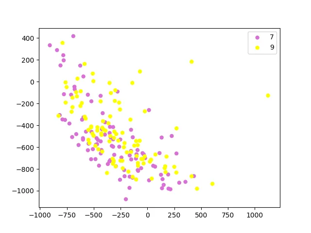
PCA projection into 2D. Pink dots are 7s, yellow dots are 9s. There’s a lot of overlap in the middle.
The two classes overlap quite a bit in two dimensions. That’s not surprising: PCA finds directions of maximum variance, not maximum class separation. The top principal components capture overall variation in digit shape (stroke width, slant, etc.), which doesn’t align perfectly with the 7-vs-9 distinction. You’d need a supervised method like LDA (linear discriminant analysis) if you wanted projections that maximize class separation.
Eigendigits#
The eigenvectors themselves live in the same 784-dimensional space as the original images, so we can reshape them back into 28x28 images. These “eigendigits” show what patterns each principal component captures:


The first eigenvector looks like a blurry average digit, which makes sense because the first principal component captures the direction of greatest overall variance. The second one picks up the contrast between the two classes. If you squint you can see how adding or subtracting these eigendigits to a mean image would push it toward looking more like a 7 or a 9.
x = eigenvectors[:,0] * 255.0
x = np.array(x, dtype='uint8').reshape(28, 28)
plt.imshow(x, cmap='gray')
plt.show()K-means clustering#
K-means is a purely unsupervised method that partitions the data into clusters by minimizing within-cluster sum of squared distances. The algorithm alternates between assigning each point to its nearest cluster centroid and recomputing centroids as the mean of their assigned points.
For classification, after running k-means on the training data, each cluster is labeled by majority vote: whichever class has more members in that cluster wins. Test points are assigned to their nearest centroid and inherit the cluster’s label.
from sklearn.cluster import KMeans

def kmeams(n):
    kmeans = KMeans(n_clusters=n, random_state=0).fit(X)
    labs = kmeans.labels_

    # Label each cluster by majority class
    cluster_labels = np.zeros(n)
    for c in range(n):
        sevens = sum(1 for i in range(1000) if labs[i] == c)
        nines = sum(1 for i in range(1000, 2000) if labs[i] == c)
        cluster_labels[c] = 7 if sevens > nines else 9

    # Predict on test set
    predictions = kmeans.predict(test_X.astype(float))
    cnt = 0
    for i in range(2000):
        expected = 7 if i < 1000 else 9
        if cluster_labels[predictions[i]] == expected:
            cnt += 1
return cnt / 2000| Clusters () | Test accuracy |
|---|---|
| 2 | 59.45% |
| 5 | 72.8% |
| 10 | 80.9% |
| 50 | 92.65% |
With , k-means basically splits the data in half along whatever direction has the most variance (similar to what PCA does). Since 7s and 9s overlap in that direction, we only get 59.45%, barely above the 50% baseline.
As increases, each cluster gets smaller and more homogeneous. With , each cluster has about 40 images on average, and most clusters end up being “pure” (all 7s or all 9s). The result: 92.65% accuracy, which is actually close to the linear SVM score (92.6%) from HW2.
The progression tells you something about the geometry of the data: 7s and 9s are not two compact blobs. They’re spread out in complicated ways through 784-dimensional space, with lots of local structure. K-means needs many small clusters to capture that structure, while a single linear boundary (SVM) or a kernel function can cut through it more efficiently.
Everything in context#
Putting all three homeworks together, here’s how the methods rank on this dataset:
| Method | Test accuracy |
|---|---|
| K-means () | 59.45% |
| K-means () | 72.8% |
| K-means () | 80.9% |
| Linear SVM | 92.6% |
| Gradient descent kernel | 92.7% |
| K-means () | 92.65% |
| Least squares classifier | 93.85% |
| Decision tree | 94.3-95.6% |
| AdaBoost | 95.1-96.25% |
| Bagging | 96.25-96.55% |
| Laplacian kernel | 97.95% |
| Gaussian kernel | 98.1% |
| Random Fourier () | 99.0% |
The story is pretty clear: linear methods top out around 93%, tree ensembles get you to 96%, and kernel methods push past 98%. K-means needs a lot of clusters to even match a linear classifier, which makes sense since it’s not actually trying to classify anything.