Bayes Classifiers, k-NN, and VC Dimension
Bayes optimal classifiers, k-NN error bounds, the curse of dimensionality in high dimensions, and VC dimension for disks and boxes.
Abstract#
The Bayes optimal classifier for discrete and continuous distributions, k-NN loss bounds, a curse of dimensionality experiment with high-dimensional Gaussians, and VC dimension analysis for disks and axis-aligned rectangles.
This was the first homework for a graduate statistical machine learning course. The problems covered the theoretical foundations that the rest of the course would build on: what does the best possible classifier look like, how does k-NN compare to it, what goes wrong in high dimensions, and how do you measure the capacity of a hypothesis class. Most of this is pen-and-paper math with a couple of coding experiments.
Bayes optimal classifier#
The setup: a feature space with three possible events , , occurring with probabilities , , . Each event has a label or with conditional probabilities:
- , so
- , so
- , so
The Bayes optimal classifier picks the label with higher posterior probability for each event. From Bayes’ rule:
Since we’re comparing posteriors for the same , the denominator cancels. We just need vs , which simplifies to comparing against directly:
- because
- because
- because
The expected loss is the probability of misclassification:
So even the best possible classifier gets 23% of the samples wrong. That’s the Bayes risk for this problem, and no classifier can beat it.
Gaussian mixture decision boundary#
Now a continuous version. A probability distribution on the real line is a mixture of two classes with densities (mean 1, variance 2) and (mean 4, variance 1), with prior probabilities 0.4 and 0.6.
The Gaussian density is:
For class +1:
For class -1:
The Bayes decision rule classifies based on which weighted density is larger. Setting and solving for gives the decision boundary at .
The Bayes decision rule: predict if , predict otherwise.
The Bayes risk is the total probability of error:
Standardizing:
And:
Total error .
Here’s what the two densities look like:
import matplotlib.mlab as mlab
import numpy as np
import matplotlib.pyplot as plt

mu1, sigma1 = 1, np.sqrt(2)
x1 = np.linspace(mu1 - 3*sigma1, mu1 + 3*sigma1, 100)
plt.plot(x1, mlab.normpdf(x1, mu1, sigma1))

mu2, sigma2 = 4, 1
x2 = np.linspace(mu2 - 3*sigma2, mu2 + 3*sigma2, 100)
plt.plot(x2, mlab.normpdf(x2, mu2, sigma2))

plt.title('Illustration of the two classes in Q2')
plt.show()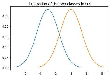
The two class densities: N(1,2) in blue and N(4,1) in orange. The overlap region around x = 2.42 is where the Bayes classifier makes errors.
k-NN expected loss#
How does k-nearest neighbors compare to the Bayes optimal? For a 2-class problem with and , the k-NN loss is:
where is a binomial random variable counting the number of the neighbors that belong to the minority class. The binomial PMF is:
The first term is the Bayes risk . The second term is always non-negative, so k-NN always does at least as badly as Bayes. For , the error is bounded by:
The upper bound also applies to 1-NN. The difference is that 3-NN can be tighter in practice because majority voting among 3 neighbors smooths out some noise. But the theoretical worst case is the same.
Note that the empirical loss of 1-NN on its own training data is always zero (each point is its own nearest neighbor), which says nothing about generalization. The 3-NN empirical loss on training data is nonzero and more informative, though still optimistic.
Curse of dimensionality#
This is where the theory meets reality. The experiment: generate 2000 points from two equally weighted spherical Gaussians and in for . Each point gets a label based on which Gaussian it came from. Train 1-NN and 3-NN classifiers, test on 1000 fresh points, and plot error rate vs. dimensionality.
Here’s the 1D case first. We generate 2000 samples from each distribution and look at their histograms:
import numpy as np
import matplotlib.pyplot as plt

NUMBER_OF_POINTS = 2000
mu1, mu2, sigma = 0, 3, 1

S1 = np.random.normal(mu1, sigma, NUMBER_OF_POINTS)
S2 = np.random.normal(mu2, sigma, NUMBER_OF_POINTS)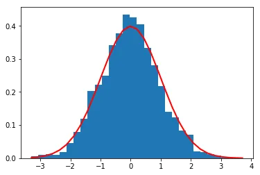
Histogram of 2000 samples from N(0,1) with the theoretical density curve overlaid in red.
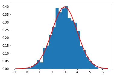
Histogram of 2000 samples from N(3,1). The two distributions are separated by 3 standard deviations.
In 1D with means 3 apart and unit variance, these distributions are well-separated. A nearest neighbor classifier should do fine. But what happens when we keep the same separation of 3 along the first axis and add dimensions?
The function that runs the experiment for arbitrary dimensionality :
from sklearn import neighbors

def test_nn(p, N_train, N_test):
    cov = np.identity(p)
    mean1 = np.zeros(p)
    mean2 = np.zeros(p)
    mean2[0] = 3

    sample1 = np.random.multivariate_normal(mean1, cov, N_train).T
    sample2 = np.random.multivariate_normal(mean2, cov, N_train).T

    X_train = np.zeros((p, N_train))
    y_train = np.zeros(N_train)

    for i in range(N_train):
        r = np.random.random_sample()
        X_train[:, i] = sample2[:, i] if r >= 0.5 else sample1[:, i]
        y_train[i] = 1 if r >= 0.5 else 0

    nbr1 = neighbors.KNeighborsClassifier(
        n_neighbors=1, algorithm='ball_tree'
    ).fit(X_train.T, y_train)
    nbr3 = neighbors.KNeighborsClassifier(
        n_neighbors=3, algorithm='ball_tree'
    ).fit(X_train.T, y_train)

    # Generate test data the same way
    sample1 = np.random.multivariate_normal(mean1, cov, N_test).T
    sample2 = np.random.multivariate_normal(mean2, cov, N_test).T

    X_test = np.zeros((p, N_test))
    y_test = np.zeros(N_test)

    for i in range(N_test):
        r = np.random.random_sample()
        X_test[:, i] = sample2[:, i] if r >= 0.5 else sample1[:, i]
        y_test[i] = 1 if r >= 0.5 else 0

    error_nn1, error_nn3 = 0, 0
    for i in range(N_test):
        y_1 = nbr1.predict(X_test[:, i].reshape(-1, 1).T).item()
        y_3 = nbr3.predict(X_test[:, i].reshape(-1, 1).T).item()
        if y_1 != y_test[i]:
            error_nn1 += 1
        if y_3 != y_test[i]:
            error_nn3 += 1

return (error_nn1 * 100.0 / N_test), (error_nn3 * 100.0 / N_test)Then loop over dimensions:
y1, y3, x = [], [], []

for i in range(11, 110, 10):
    x.append(i)
    a, b = test_nn(i, 2000, 1000)
    y1.append(a)
    y3.append(b)

plt.plot(x, y1)
plt.plot(x, y3)
plt.legend(['1-NN', '3-NN'])
plt.title('Plot of error rate vs p')
plt.show()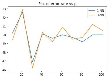
Error rates for 1-NN and 3-NN as dimensionality increases from 11 to 101. Both classifiers converge to around 50% error, which is random guessing.
Both classifiers degrade to about 50% error (random guessing) as the dimensionality goes up, even though the class means are always 3 apart along the first coordinate. This is the curse of dimensionality. In high dimensions, the distance between any two points concentrates around the same value. The signal along dimension 1 gets drowned out by the noise from the other dimensions. With 2000 training points in 101-dimensional space, the data is incredibly sparse, and nearest-neighbor distances become meaningless.
The 1-NN and 3-NN curves track each other closely, both hovering around 49-53% error for or so. Having 3 neighbors instead of 1 doesn’t help when all neighbors are equally far away.
VC dimension of disks#
VC dimension measures how complex a hypothesis class is by asking: what’s the largest set of points it can shatter (classify in all possible ways)?
For indicator functions of disks in (functions that are inside a circle, outside, but not the other way around), the analysis goes dimension by dimension.
1 point: We can always draw a disk containing the point (label ) or not containing it (label ). Trivially shattered.
2 points: Four labelings to handle. Both : draw a disk with the two points diametrically opposite. Both : any disk that misses both. One and one : center the disk on the point with radius small enough to exclude the point. All four cases work.
3 points: If they form a triangle, the circumcircle passes through all three (all ). For cases with one or two s, we can shrink or shift the disk to include only the points. All : any disk avoiding all three. This works for all 8 labelings.
4 points: Here it breaks. Consider four points forming a quadrilateral. Take the labeling where one pair of diagonal points is and the other pair is . Any disk containing the two points (which are diagonal) would have to stretch across the quadrilateral, and the two points (also diagonal) would fall inside. If you flip which diagonal pair is , you hit the same problem from the other direction. You can’t separate diagonal pairs with a convex region.
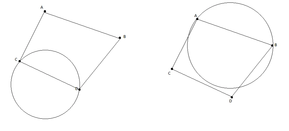
Attempting to shatter 4 points with circles. When trying to include opposite diagonal points while excluding the other diagonal, the circle must be too large to avoid the excluded points.
So the VC dimension with invertible indicator functions (can be inside or inside) would be 3.
But the problem specifies one-sided indicators only: inside, outside, never the reverse. With this restriction, even 3 collinear points can’t be shattered. Place 3 points on a line with the middle one labeled and the outer two labeled . No disk can contain both outer points without also containing the middle one, because disks are convex.
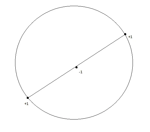
Three collinear points with labels +1, -1, +1. No circle can contain both outer points without containing the middle one, since circles are convex.
With the one-sided restriction, the VC dimension is 2.
VC dimension of axis-aligned rectangles#
For indicator functions of axis-aligned rectangular boxes in ( inside the box, outside):
1 point: Trivial. Box around it for , box elsewhere for .
2 points: All 4 labelings work. We can make a box containing any subset of the two points.
3 points: Any triangle formed by 3 points can be enclosed in an axis-aligned bounding box. For subsets, we can make tighter boxes that include only the desired points. All 8 labelings are achievable.
4 points: Assign the points to roles by their extremal positions: topmost, bottommost, leftmost, rightmost. (If a point is both leftmost and topmost, some cases degenerate to fewer than 4 distinct extreme points, which reduces to the 3-point case.) For 4 distinct extreme points, the bounding box with width from leftmost to rightmost and height from bottommost to topmost contains all four. Any subset of 1, 2, or 3 points can be enclosed by adjusting the box boundaries. The empty set is just a box that misses all points. All 16 labelings work.
5 points: With 5 points, at least one point must lie inside the bounding box defined by the other four extreme points (top, bottom, left, right). You can’t label that interior point as while labeling all four boundary-defining points as , because the bounding box that contains the four extremal points necessarily contains the interior point too.
The VC dimension is 4.
The jump from 3 (for disks) to 4 (for rectangles) makes sense geometrically. Rectangles have 4 independent parameters (left, right, top, bottom edges), while circles have 3 (center x, center y, radius). VC dimension tends to track the number of free parameters, though that’s a heuristic, not a theorem.