
Word2Vec from Scratch
Building skip-gram and CBOW word2vec models with negative sampling, training on the Stanford Sentiment Treebank.
Abstract#
Implement word2vec (skip-gram and CBOW) with negative sampling from scratch using NumPy, including softmax, sigmoid, gradient checking, backpropagation, and SGD. Train word vectors on the Stanford Sentiment Treebank and visualize the learned embeddings.
This was the biggest assignment in the course. It started with building basic neural network components (softmax, sigmoid, a two-layer backprop network) and worked up to a full word2vec implementation with skip-gram, CBOW, and negative sampling. The whole thing runs on NumPy only.
Neural network basics#
Softmax#
The softmax function converts a vector of raw scores into a probability distribution:
A useful property: softmax is invariant to constant offsets. Adding any constant to every element gives the same output: . We use this for numerical stability by subtracting the row maximum before exponentiating, which prevents overflow in np.exp:
def softmax(x):
    X_ = np.atleast_2d(x)
    X_ -= np.max(X_, axis=1).reshape(-1, 1)
    X_ = np.exp(X_)
    X_ /= np.sum(X_, axis=1).reshape(-1, 1)
    if len(x.shape) == 1:
        x = X_.flatten()
    else:
        x = X_
return xThe function handles both 1-D vectors and 2-D matrices (applying softmax row-by-row).
Sigmoid#
Same sigmoid from the logistic regression assignment:
with input clipping for numerical stability, and the gradient .
Gradient checking#
Also the same centered difference approach from before: perturb each parameter by , compute the numerical gradient as , and compare against the analytical gradient. All gradient checks passed throughout the assignment (six total: three for basic functions, one for the neural network, and two for word2vec models).
Two-layer neural network#
The backpropagation section has you build a small neural network with architecture 10 5 10: ten input units, five hidden units with sigmoid activation, and ten output units with softmax and cross-entropy loss.
The forward pass:
The backward pass computes gradients using the chain rule:
Then the weight gradients are just matrix multiplications of the layer inputs with the deltas. The gradient check passed on random data with 20 samples.
Word2Vec#
Word2vec learns dense vector representations for words by training a model to predict context words from a center word (skip-gram) or a center word from its context (CBOW). The key idea is that words appearing in similar contexts should have similar vectors.
Softmax cost function#
The full softmax cost for word2vec computes the probability of the target word given center word :
where is the input (center) vector and is the output (context) vector. This requires summing over the entire vocabulary for the denominator, which is expensive.
def softmaxCostAndGradient(predicted, target, outputVectors, dataset):
    y_hat = softmax(outputVectors.dot(predicted))
    cost = -np.log(y_hat[target])
    # Gradients computed analytically
return cost, gradPred, gradNegative sampling#
To avoid the expensive sum over the whole vocabulary, negative sampling approximates the cost by contrasting the true context word against randomly sampled “negative” words:
The first term pushes the true context word’s vector closer to the center word. The second term pushes random words away. We used negative samples.
def negSamplingCostAndGradient(predicted, target, outputVectors, dataset, K=10):
    # Sample K negative indices != target
    indices = [target]
    for k in range(K):
        newidx = dataset.sampleTokenIdx()
        while newidx == target:
            newidx = dataset.sampleTokenIdx()
        indices.append(newidx)

    # Cost and gradient computation using sigmoid
    # Uses np.add.at for accumulating gradients at repeated indices
return cost, gradPred, gradOne detail: np.add.at is needed because the same negative word might get sampled more than once. Normal indexing with += wouldn’t accumulate correctly in that case.
Skip-gram and CBOW#
Skip-gram predicts each context word independently given the center word. For a center word with context words , it sums the cost and gradients from each (center, context) pair:
def skipgram(currentWord, C, contextWords, tokens,
             inputVectors, outputVectors, dataset,
             word2vecCostAndGradient=softmaxCostAndGradient):
    cost = 0.0
    gradIn = np.zeros(inputVectors.shape)
    gradOut = np.zeros(outputVectors.shape)
    for j in contextWords:
        c, gi, go = word2vecCostAndGradient(
            inputVectors[tokens[currentWord]], tokens[j],
            outputVectors, dataset)
        cost += c
        gradIn[tokens[currentWord]] += gi
        gradOut += go
return cost, gradIn, gradOutCBOW (Continuous Bag of Words) goes the other direction: predict the center word from the context. It sums all the context word vectors into a single predicted vector and makes one prediction:
def cbow(currentWord, C, contextWords, tokens,
         inputVectors, outputVectors, dataset,
         word2vecCostAndGradient=softmaxCostAndGradient):
    predicted = np.zeros(inputVectors.shape[1])
    for j in contextWords:
        predicted += inputVectors[tokens[j]]
    cost, gradPred, gradOut = word2vecCostAndGradient(
        predicted, tokens[currentWord], outputVectors, dataset)
    gradIn = np.zeros(inputVectors.shape)
    for j in contextWords:
        gradIn[tokens[j]] += gradPred
return cost, gradIn, gradOutSGD and training#
The SGD implementation includes learning rate annealing (halving the rate every 20,000 iterations) and saves parameters every 1,000 iterations:
def sgd(f, x0, step, iterations, postprocessing=None,
        useSaved=False, PRINT_EVERY=10):
    ANNEAL_EVERY = 20000
    for iter in range(iterations):
        cost, grad = f(x0)
        x0 -= step * grad
        if iter % ANNEAL_EVERY == 0 and iter > 0:
            step *= 0.5
return x0The training setup:
- Dataset: Stanford Sentiment Treebank
- Model: Skip-gram with negative sampling ()
- Vector dimensions: 10
- Context window: (random window size from 1 to )
- Learning rate: 0.3, halved at iteration 20,000
- Iterations: 40,000
- Batch size: 50 (per SGD step, sample 50 random center words)
The word vectors are initialized with small random values for the input vectors and zeros for the output vectors. After training, the final word vectors are the sum of input and output vectors.
Training cost over time:
| Iteration | Cost |
|---|---|
| 10 | ~20.3 |
| 5,000 | ~17.4 |
| 10,000 | ~12.7 |
| 20,000 | ~10.7 |
| 30,000 | ~9.9 |
| 40,000 | ~9.4 |
The cost dropped from about 20 to about 9.4 over 40,000 iterations. The assignment said it should be “around or below 10,” so this was a pass.
Visualization#
To see what the word vectors learned, we project them down to 2D using SVD (similar to PCA). The visualization plots 25 selected words:
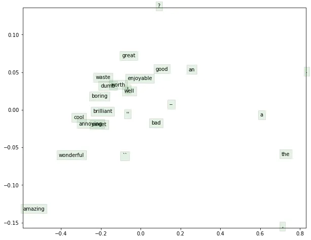
Word vectors projected to 2D via SVD, trained on the Stanford Sentiment Treebank. Positive sentiment words (good, great, cool, brilliant, wonderful, amazing, worth, sweet, enjoyable) cluster together. Negative sentiment words (boring, bad, waste, dumb, annoying) form their own cluster. Function words and punctuation land in separate regions.
The clusters make sense. The model was trained on a sentiment dataset, so it saw words like “good” and “great” in similar contexts (positive movie reviews) and words like “bad” and “boring” in similar contexts (negative reviews). The vectors reflect that: words with similar usage patterns end up near each other in the embedding space. Punctuation and function words (“the”, “a”, “an”, commas, periods) sit in their own clusters because they appear in all kinds of contexts regardless of sentiment.
Even with only 10-dimensional vectors trained for 40,000 iterations on a relatively small dataset, the model picks up on the sentiment distinction. That’s the core promise of word2vec: you don’t need labeled data or hand-crafted features. Just predict context words, and the learned representations capture meaning.