RBF Networks for Function Approximation

Second project for CSE 5526: Introduction to Neural Networks (Autumn 2018). After implementing an MLP with backpropagation in Project 1, this project had us build a Radial Basis Function (RBF) network, which is a pretty different kind of architecture.

The Problem: Function Approximation with Noise#

The target function is a noisy sinusoid:

$h(x) = 0.5 + 0.4 \sin(2\pi x)$

Training data consists of 75 random points sampled uniformly from $[0, 1]$, with additive uniform noise in $[-0.1, 0.1]$. The task is to learn an approximation of $h(x)$ from this noisy data.

It’s a nice benchmark because the true function is simple enough to visualize, but the noise and random sampling mean the network has to actually generalize instead of just memorizing the training points.

RBF Network Architecture#

Where MLPs use sigmoid activations and train everything end-to-end with backpropagation, RBF networks take a different approach:

1. Basis layer: Each basis function is a Gaussian centered at a specific point in input space:

$\phi_i(x) = \exp\left(-\frac{(x - \mu_i)^2}{2\sigma_i^2}\right)$

2. Output layer: A linear combination of the basis function outputs:

$y(x) = \sum_{i=1}^{K} w_i \phi_i(x) + b$

The basis functions are local: each one responds strongly only to inputs near its center $\mu_i$, with the spread controlled by the width $\sigma_i$. The output layer then just learns a linear combination of these local responses.

Training: K-Means + LMS#

Training happens in two separate phases, which is one of the big differences from an MLP.

Phase 1: Unsupervised Center Selection via K-Means#

The Gaussian centers $\mu_i$ are found by running K-Means clustering on the training inputs. This is entirely unsupervised: the desired outputs don’t factor in at all. K-Means partitions the input space into $K$ clusters, and each cluster centroid becomes a basis function center.

def kmeans(X, clusters, isSameWidth):
    centers = np.random.choice(np.squeeze(X), clusters, False)
    centers = centers.reshape(clusters, 1)
    while True:
        dist = np.array([euc_dist(X, centers[i]) for i in range(clusters)])
        predicted = np.argmin(np.squeeze(dist).T, axis=1)
        centers_new = np.array([np.mean(X[predicted == i], axis=0)
                                for i in range(clusters)])
        if np.array_equal(centers_new, centers):
            break
        centers = centers_new
    return centers

Gaussian Width Strategies#

Two strategies for setting the widths $\sigma_i$ were compared:

Same width (shared): All basis functions use a single width derived from the spread of the centers:

$\sigma = \frac{\max(\mu) - \min(\mu)}{\sqrt{2K}}$

Different width (per-cluster): Each basis function’s width is the RMS distance of its assigned training points to its center:

$\sigma_i = \sqrt{\frac{1}{|S_i|} \sum_{x \in S_i} (x - \mu_i)^2}$

If a center has no assigned points, its width defaults to the mean of the other widths.

Phase 2: Supervised Weight Training via LMS#

With the centers and widths fixed, the output weights are trained using the Least Mean Squares (LMS) rule, which is just online gradient descent, updating after each sample:

$W \leftarrow W + \eta \cdot \phi(x) \cdot (d - y)$ $b \leftarrow b + \eta \cdot (d - y)$

Training runs for 100 epochs over the 75 training points.

Experimental Setup#

I swept across 20 configurations:

• Number of bases (K): 2, 4, 7, 11, 16
• Learning rate ($\eta$): 0.01, 0.02
• Gaussian width strategy: same, different

Results and Analysis#

Effect of Gaussian Width Strategy#

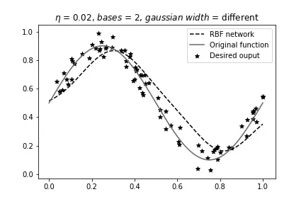
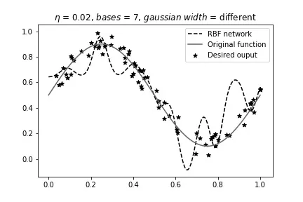
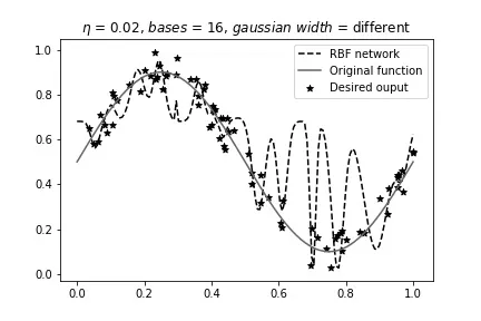
This turned out to be the most important factor. With per-cluster (different) widths, the network overfits badly, especially as $K$ increases. Each basis function adapts its width to its local cluster, which can create narrow, spiky responses that chase individual data points instead of capturing the underlying sinusoidal trend.

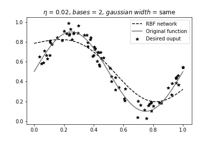
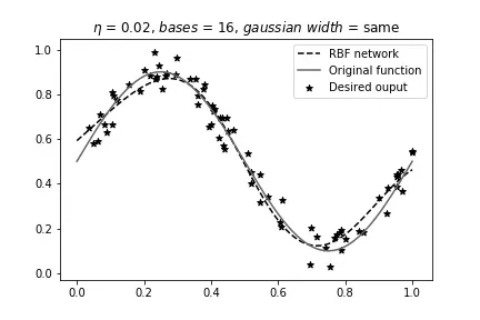
With shared (same) width, the network produces smoother approximations. Constraining all basis functions to operate at the same scale acts as a form of regularization. The network holds form well up to about $K = 7$.

Here are some comparisons at $\eta = 0.02$:

Same width, 2 bases (best overall result):

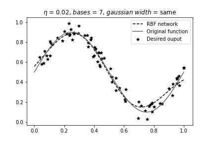
Same width, 7 bases (starting to get complicated):

Same width, 16 bases (overfitting despite shared width):

Now the per-cluster width variant at the same configurations:

Different width, 2 bases:

Different width, 7 bases:

Different width, 16 bases:

Effect of Learning Rate#

Changing $\eta$ from 0.01 to 0.02 didn’t affect the overall trends much. The main difference showed up at high $K$ with variable widths, where the higher learning rate caused more pronounced oscillations. For the well-behaved configurations (low $K$, same width), both learning rates gave nearly identical results.

Best Configuration#

The best results came from $\eta = 0.02$ with 2 bases, regardless of width strategy. At this low model complexity, both width strategies produce similar results because two basis functions don’t have enough degrees of freedom to overfit. I’d personally prefer the shared-width variant though, since it generalizes more robustly as $K$ increases.

What I Took Away#

The big thing with RBF networks is how the training splits into two independent phases: unsupervised center selection (K-Means) and then supervised weight training (LMS). The representation is fixed before the output weights are ever touched, which is conceptually simpler than backpropagation where everything gets optimized jointly, but it also means you’re stuck with whatever representation K-Means gives you.

The results were a clean demonstration of the bias-variance tradeoff. With 75 noisy samples from a simple sinusoid, 2 basis functions are enough. Adding more bases just gives the network more capacity to memorize noise.

The shared vs. per-cluster width comparison was maybe the most interesting part. Forcing all Gaussian widths to be the same is a constraint that limits what the network can do, but it actually improves generalization by preventing individual basis functions from getting too narrow and spiking at specific data points. Sometimes less flexibility gives you better results.

One thing I liked about RBF networks over MLPs is that you can actually see what’s going on. Each basis function has a center and a width in input space, so when the network overfits you can literally see narrow Gaussians spiking up at individual data points while ignoring the broader trend. That kind of interpretability was helpful for building intuition about what overfitting actually looks like.