Shape Moments and PCA on a Box of Dots • TheAnig

Abstract#

Two separate problems. The first computes spatial, central, and similitude moments on binary rectangle images. Most of the eta values come out to zero because the rectangles are perfectly symmetric, which is the point. The second does PCA on a 2D point cloud: mean subtraction, eigendecomposition of the covariance matrix, confidence ellipses, decorrelation, and projection down to 1D. The PCA part was more interesting than the moments.

Similitude moments#

Image moments are scalar quantities computed from the pixel coordinates and intensities. There are three levels. Spatial moments depend on position and scale. Central moments subtract the mean, making them translation-invariant. Similitude moments normalize by $m_{00}$ on top of that, so they’re invariant to both translation and scale.

The function computes all three levels and returns them in a dictionary. I used numpy.mgrid to build coordinate grids for $x$ and $y$ :

def similitudeMoments(image):

    assert len(image.shape) == 2

    x, y = mgrid[:image.shape[0], :image.shape[1]]

    moments = {}

    moments['mean_x'] = sum(x * image) / sum(image)
    moments['mean_y'] = sum(y * image) / sum(image)

    # Spatial moments
    moments['m00'] = sum(image)

    moments['m01'] = sum(x * image)
    moments['m10'] = sum(y * image)

    moments['m11'] = sum(y * x * image)
    moments['m02'] = sum(x**2 * image)
    moments['m20'] = sum(y**2 * image)

    moments['m12'] = sum(x * y**2 * image)
    moments['m21'] = sum(x**2 * y * image)
    moments['m03'] = sum(x**3 * image)
    moments['m30'] = sum(y**3 * image)

    # Central moments (translation invariant)
    moments['mu11'] = sum((x - moments['mean_x']) *
                          (y - moments['mean_y']) * image)
    moments['mu02'] = sum((y - moments['mean_y'])**2 * image)
    moments['mu20'] = sum((x - moments['mean_x'])**2 * image)

    moments['mu12'] = sum((x - moments['mean_x']) *
                          (y - moments['mean_y'])**2 * image)
    moments['mu21'] = sum((x - moments['mean_x'])**2 *
                          (y - moments['mean_y']) * image)
    moments['mu03'] = sum((y - moments['mean_y'])**3 * image)
    moments['mu30'] = sum((x - moments['mean_x'])**3 * image)

    # Similitude moments (translation + scale invariant)
    # eta_pq = mu_pq / m00^((p+q)/2 + 1)
    moments['eta11'] = moments['mu11'] / sum(image)**(2/2 + 1)
    moments['eta12'] = moments['mu12'] / sum(image)**(3/2 + 1)
    moments['eta21'] = moments['mu21'] / sum(image)**(3/2 + 1)
    moments['eta02'] = moments['mu02'] / sum(image)**(2/2 + 1)
    moments['eta20'] = moments['mu20'] / sum(image)**(2/2 + 1)
    moments['eta03'] = moments['mu03'] / sum(image)**(3/2 + 1)
    moments['eta30'] = moments['mu30'] / sum(image)**(3/2 + 1)

    return moments

python

The normalization formula is:

$\eta_{pq} = \frac{\mu_{pq}}{m_{00}^{(p+q)/2 + 1}}$

The test images are four BMPs of white rectangles on black backgrounds (boxIm1.bmp through boxIm4.bmp). Three are oriented the same way, one is transposed.

image_cube = []
for i in range(1, 5):
    tmp = imread(f'./data/boxIm{i}.bmp')
    tmp = img_as_float(tmp)
    image_cube.append(tmp)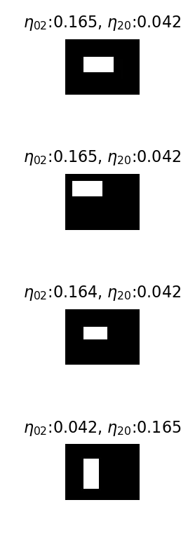

python

Four box images with eta moment values — Each box image with its $\eta_{02}$ and $\eta_{20}$ values.

Every eta moment except $\eta_{02}$ and $\eta_{20}$ comes out to 0. The rectangles are perfectly symmetric, so there’s no skewness ( $\eta_{03}$ , $\eta_{30}$ = 0), no cross-correlation ( $\eta_{11}$ = 0), nothing. The only thing the moments capture is the spread along each axis, which is what $\eta_{02}$ and $\eta_{20}$ measure.

For the one rectangle that’s oriented transversely, the $\eta_{02}$ and $\eta_{20}$ values swap. That’s the moment representation saying “the shape is the same, just rotated 90 degrees.”

Eigenanalysis of 2D data#

Second part of the assignment: load eigdata.txt, a 2D point cloud, and do PCA on it.

X = np.loadtxt('./data/eigdata.txt')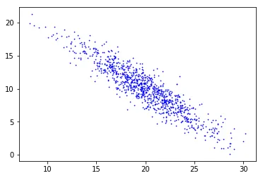

python

Raw scatter plot of eigdata — Raw data from eigdata.txt. There’s a clear elongated structure tilted off-axis.

The first step is mean subtraction. Center the data at the origin.

m = np.mean(X, axis=0)
Y = X - m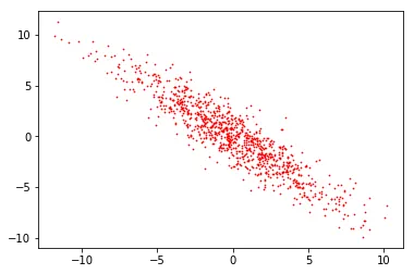

python

Mean-subtracted scatter plot — After subtracting the mean. Same shape, centered at (0, 0).

Covariance and eigenvectors#

Compute the covariance matrix of the mean-subtracted data and decompose it:

covariance = np.cov(Y.T)
[w, v] = np.linalg.eig(covariance)

largest_eigvec = v[0]
smallest_eigvec = v[1]

python

(Note: I used np.linalg.eig(covariance), not np.linalg.inv(covariance). This changes the subsequent steps slightly.)

The eigenvalues tell you how much variance there is along each eigenvector, and the eigenvectors themselves give the directions. To visualize the spread, I drew a $3\sigma$ confidence ellipse around the data.

The $3\sigma$ confidence interval corresponds to 0.9973, and the $\chi^2$ value for 2 degrees of freedom at that level is 7.378. The semi-axes of the ellipse are $\sqrt{\chi^2} \cdot \sqrt{\lambda}$ where $\lambda$ is each eigenvalue.

chisquare_val = np.sqrt(7.378)
theta_grid = np.linspace(0, 2 * np.pi)

angle = np.arctan2(largest_eigvec[1], largest_eigvec[0])
if angle < 0:
    angle = angle + 2 * np.pi

phi = -angle

a = chisquare_val * np.sqrt(w[0])
b = chisquare_val * np.sqrt(w[1])

ellipse_x_r = a * np.cos(theta_grid)
ellipse_y_r = b * np.sin(theta_grid)

python

The rotation matrix aligns the ellipse with the eigenvectors:

R = np.array([
    [np.cos(phi), np.sin(phi)],
    [-np.sin(phi), np.cos(phi)]
]).reshape((2, 2))

r_ellipse = np.vstack((ellipse_x_r, ellipse_y_r)).T @ R

python

plt.plot(r_ellipse[:, 0] + X0, r_ellipse[:, 1] + Y0, c='#db2f27')
plt.scatter(Y[:, 0], Y[:, 1], s=0.5, c='#008cbc')
plt.quiver(0, 0, -1.5*np.sqrt(largest_eigvec),
           1*np.sqrt(largest_eigvec), color='#007500', scale=3.4)
plt.quiver(0, 0, 1*np.sqrt(smallest_eigvec),
           1.5*np.sqrt(smallest_eigvec), color='#0b3954', scale=15)

python

The np.sqrt(smallest_eigvec) call throws a RuntimeWarning: invalid value encountered in sqrt because eigenvector components can be negative. The quiver arrows still render fine, the NaN components just get ignored.

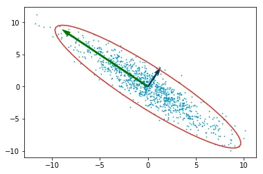
Scatter with 3-sigma ellipse and eigenvector arrows — Mean-subtracted data with $3\sigma$ confidence ellipse (red) and eigenvector arrows (green = largest, dark blue = smallest).

The green arrow points along the direction of maximum variance. The dark blue arrow is perpendicular to it.

Decorrelation#

Decorrelation: divide the mean-subtracted data by the per-axis standard deviation, then multiply by the eigenvector matrix. This rotates the data so the principal axes line up with the coordinate axes.

stddev = np.sqrt(np.diag(covariance))
decorrelated_y = np.divide(Y, stddev)
decorrelated_y = decorrelated_y @ v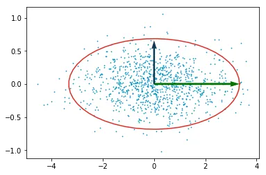

python

Decorrelated data with ellipse — Decorrelated data. The principal axes now align with the coordinate axes.

The ellipse looks fatter here than in the previous plot. It’s not. The axis scaling is different because I adjusted it to make the plot readable. If you measured the actual semi-axis ratios they’d be the same.

1D projection#

Last step: project the mean-subtracted data onto the largest eigenvector. This collapses 2D down to 1D.

projected_y = Y @ largest_eigvec.T
plt.scatter(projected_y, np.zeros_like(projected_y), c='blue')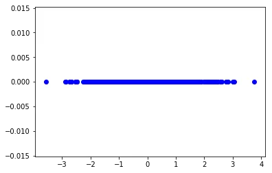

python

1D projection onto largest eigenvector — Data projected onto the largest eigenvector. All points collapsed to a single axis.

Some information is lost along the minor axis, but the data was already elongated in one direction, so the loss is small.

At 2 dimensions, PCA works fine. With higher-dimensional data you’d want to compare against something like t-SNE to see if there’s nonlinear structure that PCA misses.